MATLAB에서 TensorFlow 호출하기

Note: All comments and opinions expressed on "MATLAB for everyone" are mine alone and do not necessarily reflect those of my employers, past or present.

본 게시글의 원문은 Yann Debray의 MATLAB with Python Book 입니다. 해당 책은 MIT 라이센스를 따르기 때문에 개인적으로 번역하여 재배포 합니다. 본 포스팅에는 추후 유료 수익을 위한 광고가 부착될 수도 있습니다.

MIT License

Copyright (c) 2023 Yann Debray

Permission is hereby granted, free of charge, to any person obtaining a copy
of this software and associated documentation files (the "Software"), to deal
in the Software without restriction, including without limitation the rights
to use, copy, modify, merge, publish, distribute, sublicense, and/or sell
copies of the Software, and to permit persons to whom the Software is
furnished to do so, subject to the following conditions:

The above copyright notice and this permission notice shall be included in all
copies or substantial portions of the Software.

THE SOFTWARE IS PROVIDED "AS IS", WITHOUT WARRANTY OF ANY KIND, EXPRESS OR
IMPLIED, INCLUDING BUT NOT LIMITED TO THE WARRANTIES OF MERCHANTABILITY,
FITNESS FOR A PARTICULAR PURPOSE AND NONINFRINGEMENT. IN NO EVENT SHALL THE
AUTHORS OR COPYRIGHT HOLDERS BE LIABLE FOR ANY CLAIM, DAMAGES OR OTHER
LIABILITY, WHETHER IN AN ACTION OF CONTRACT, TORT OR OTHERWISE, ARISING FROM,
OUT OF OR IN CONNECTION WITH THE SOFTWARE OR THE USE OR OTHER DEALINGS IN THE
SOFTWARE.

본 게시물에서 활용된 소스 코드들은 모두 Yann Debray의 GitHub Repo에서 확인할 수 있습니다.

5.2. MATLAB에서 TensorFlow 호출하기

TensorFlow를 사용하는 방법을 소개하겠습니다. 시작 가이드 튜토리얼을 통해 진행해보겠습니다:

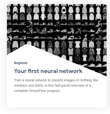
이 가이드에서는 10개의 카테고리에 속하는 70,000개의 흑백 이미지를 포함하는 Fashion MNIST 데이터셋을 사용합니다.

이 이미지들은 낮은 해상도(28 x 28 픽셀)에서 개별 의류 아이템을 나타냅니다.

이 예제는 Zalando에서 제작한 것으로 MIT 라이선스에 따릅니다.

먼저, TensorFlow를 로드하고 설치된 TensorFlow 버전을 확인해보겠습니다:

tf = py.importlib.import_module('tensorflow');
pyrun('import tensorflow as tf; print(tf.__version__)')

2.8.0

그런 다음 데이터셋을 가져오겠습니다.

fashion_mnist = tf.keras.datasets.fashion_mnist

fashion_mnist = 
  Python module with properties:

    load_data: [1x1 py.function]

    <module 'keras.api._v2.keras.datasets.fashion_mnist' from 'C:\\Users\\ydebray\\AppData\\Local\\WPy64-39100\\python-3.9.10.amd64\\lib\\site-packages\\keras\\api\\_v2\\keras\\datasets\\fashion_mnist\\__init__.py'>

train_test_tuple = fashion_mnist.load_data();

그리고 훈련 및 테스트용 이미지와 레이블을 따로 저장하겠습니다.

Python 튜플을 MATLAB에서 인덱싱할 때 중괄호를 사용합니다: pytuple{1}

(MATLAB은 1부터 시작하는 인덱스를 사용하므로 Python과 달리 주의해야 합니다)

% ND array containing gray scale images (values from 0 to 255)
train_images = train_test_tuple{1}{1}; 
test_images = train_test_tuple{2}{1};
% values from 0 to 9: can be converted as uint8
train_labels = train_test_tuple{1}{2};
test_labels = train_test_tuple{2}{2}; 

MATLAB에서 클래스 목록을 직접 정의합니다:

class_names = ["T-shirt/top", "Trouser", "Pullover", "Dress", "Coat", "Sandal", "Shirt", "Sneaker", "Bag", "Ankle boot"];

class_names = 1x10 string    
"T-shirt/top""Trouser"    "Pullover"   "Dress"      "Coat"       "Sandal"     "Shirt"      "Sneaker"    "Bag"        "Ankle boot"

만약 MATLAB에서 위의 목록에서 훈련 레이블의 인덱스를 사용하려면 [0:9] 범위를 [1:10] 범위로 변경해야 합니다.

tl = uint8(train_labels)+1; % [0:9] 범위를 [1:10] 범위로 변경
l = length(tl)

l = 60000

다음은 훈련 세트에 60,000개의 이미지가 있으며 각 이미지가 28 x 28 픽셀로 표시됨을 나타냅니다.

train_images_m = uint8(train_images);
size(train_images_m)

ans = 1x3    
       60000          28          28

단일 이미지의 크기를 변경하려면 reshape 함수를 사용합니다:

size(train_images_m(1,:,:))

ans = 1x3    
     1    28    28

size(reshape(train_images_m(1,:,:),[28,28]))

ans = 1x2    
    28    28

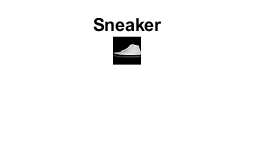
데이터셋을 탐색하도록 라이브 스크립트에 라이브 컨트롤을 추가할 수 있습니다.

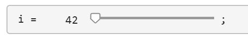
i = 42;
img = reshape(train_images_m(i,:,:),[28,28]);
imshow(img)
title(class_names(tl(i)))

figure_0

신경망을 훈련하기 전에 데이터를 전처리해야 합니다.

만약 훈련 데이터 세트의 첫 번째 이미지를 살펴보면, 픽셀 값이 0부터 255 사이의 범위에 있다는 것을 알 수 있습니다:

train_images = train_images / 255;
test_images = test_images / 255;

마지막으로, tf_helper 파일 또는 모듈에서 지정한 함수로 모델을 구축하고 훈련할 수 있습니다:

model = py.tf_helper.build_model();

모델의 아키텍처를 확인하려면 셀 배열에서 레이어를 검색할 수 있습니다:

cell(model.layers)

	1	2	3
1	1x1 Flatten	1x1 Dense	1x1 Dense

py.tf_helper.compile_model(model);
py.tf_helper.train_model(model,train_images,train_labels) 

Epoch 1/10

   1/1875 [..............................] - ETA: 12:59 - loss: 159.1949 - accuracy: 0.2500
  39/1875 [..............................] - ETA: 2s - loss: 52.8977 - accuracy: 0.5256    
  76/1875 [>.............................] - ETA: 2s - loss: 34.8739 - accuracy: 0.6049
 113/1875 [>.............................] - ETA: 2s - loss: 28.4213 - accuracy: 0.6350
 157/1875 [=>............................] - ETA: 2s - loss: 22.9735 - accuracy: 0.6616
 194/1875 [==>...........................] - ETA: 2s - loss: 20.3405 - accuracy: 0.6740
 229/1875 [==>...........................] - ETA: 2s - loss: 18.3792 - accuracy: 0.6861
 265/1875 [===>..........................] - ETA: 2s - loss: 16.7848 - accuracy: 0.6943

 ...

테스트 데이터 세트에서 모델의 성능을 평가하여 모델을 평가합니다.

test_tuple = py.tf_helper.evaluate_model(model,test_images,test_labels)

313/313 - 0s - loss: 0.5592 - accuracy: 0.8086 - 412ms/epoch - 1ms/step
test_tuple = 
  Python tuple with values:

    (0.5592399835586548, 0.8086000084877014)

    Use string, double or cell function to convert to a MATLAB array.

test_acc = test_tuple{2}

test_acc = 0.8086

테스트 데이터 세트의 첫 번째 이미지에 대해 모델을 테스트해보세요:

test_images_m = uint8(test_images);
prob = py.tf_helper.test_model(model,py.numpy.array(test_images_m(1,:,:)))

prob = 
  Python ndarray:

    0.0000    0.0000    0.0000    0.0000    0.0000    0.0002    0.0000    0.0033    0.0000    0.9965

    Use details function to view the properties of the Python object.

    Use single function to convert to a MATLAB array.

[argvalue, argmax] = max(double(prob))

argvalue = 0.9965
argmax = 10

imshow(reshape(test_images_m(1,:,:),[28,28])*255)
title(class_names(argmax))